Calibration Plot for Football Predictions

Why calibration is different from accuracy

Accuracy looks only at the model’s most likely outcome.

Suppose two models both predict 100 matches and select the correct result 60 times.

Their accuracy is identical at 60%.

But imagine Model A usually assigns probabilities around 50% to 60%, while Model B routinely assigns 85% or 90% to the same selections.

Those models are making very different claims about uncertainty.

If the outcomes labelled 90% only happen 70% of the time, Model B is overconfident even if its top pick remains correct more often than not.

Calibration asks whether those probability statements are trustworthy.

This matters whenever the probability itself is used downstream, including expected-value calculations, risk models, rankings or staking systems.

Accuracy cannot tell you that a 70% prediction behaves like a real 70%.

A calibration plot can.

How to read a calibration plot for match predictions

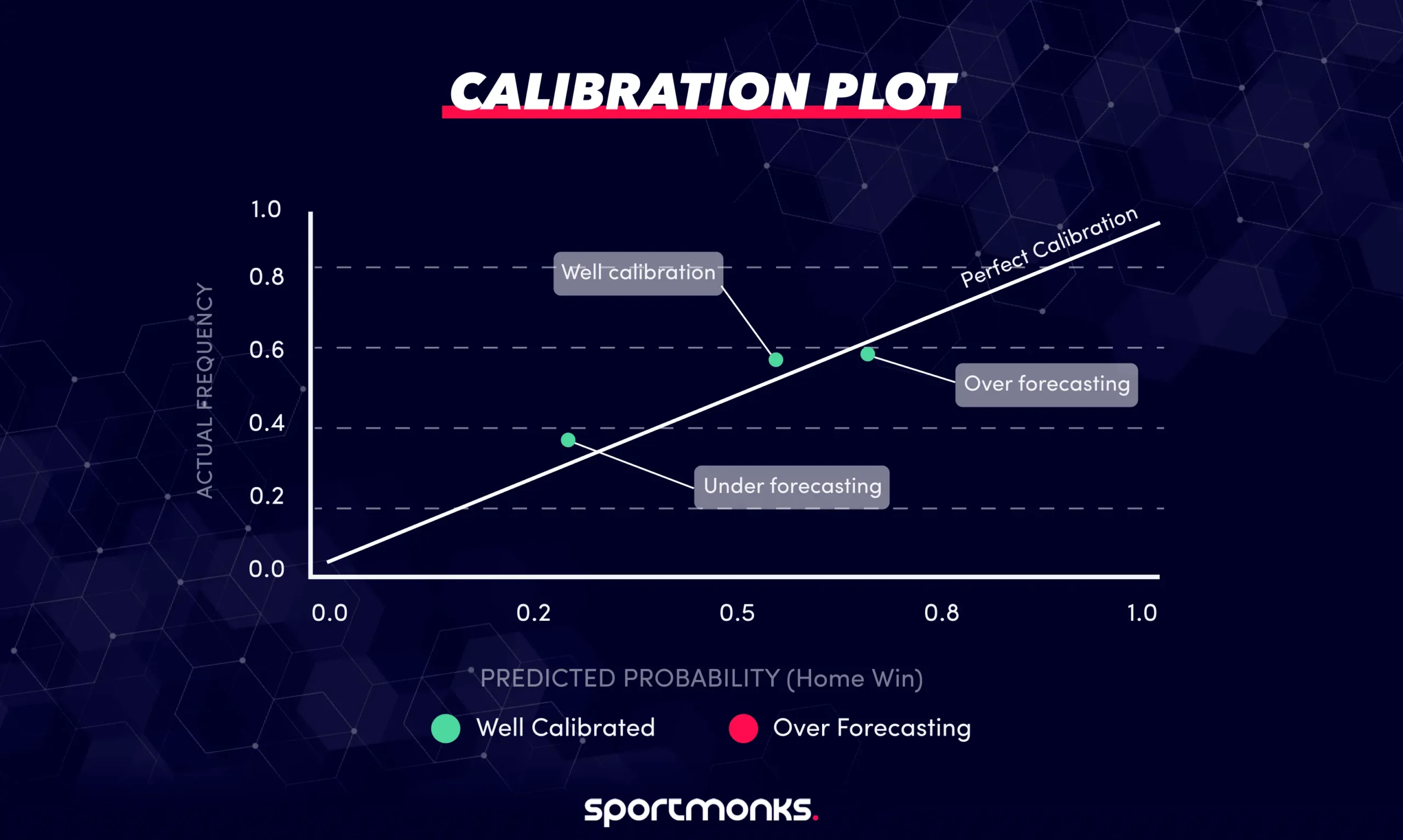
A calibration plot groups predictions into probability ranges, then compares the model’s average predicted probability with the actual observed frequency.

For example, you might use bins such as:
– 0% to 10%.
– 10% to 20%.
– 20% to 30%.
– 30% to 40%.
– 40% to 50%.
– 50% to 60%.
– 60% to 70%.
– 70% to 80%.
– 80% to 90%.
– 90% to 100%.

Each bin becomes a point on the chart.

The x-axis represents the model’s average predicted probability.

The y-axis represents how often the outcome actually happened.

A perfectly calibrated model would follow the diagonal line from the bottom-left to the top-right.
– Points on or close to the diagonal indicate that predicted probability and observed frequency are similar.
– Points below the diagonal indicate over-forecasting. The model assigns a higher probability than the outcome actually achieves.
– Points above the diagonal indicate under-forecasting. The outcome happens more often than the model predicts.

The important question is not whether every point lands exactly on the diagonal. Sampling noise means that is unlikely.

Look instead for consistent patterns across several bins.

A worked calibration example

Suppose your model assigns home-win probabilities across an entire league season.

One of the bins contains 180 matches.

The average predicted home-win probability in that bin is:

0.648

Home teams actually win 115 of those matches.

The observed frequency is therefore:

115 / 180 = 0.639

The difference is small:

Predicted: 64.8% 
Observed: 63.9%

That point would sit close to the diagonal.

Now imagine another probability range contains 40 matches with an average prediction of 84%.

Only 29 of those matches produce the predicted outcome.

The observed frequency is:

29 / 40 = 72.5%

That bin would sit below the diagonal because the model predicted 84% but the outcome occurred only 72.5% of the time.

This does not prove that all high-confidence football predictions are systematically overconfident.

It tells you that this model, in this dataset and probability range, appears overconfident.

That is the kind of pattern a calibration plot is designed to expose.

Building calibration bins in Python

A simple calibration function can divide predictions into equal-width probability bins.

import numpy as np
import pandas as pd


def calibration_bins(
    y_true,
    y_prob,
    n_bins=10,
):
    bins = np.linspace(
        0,
        1,
        n_bins + 1,
    )

    bin_ids = np.digitize(
        y_prob,
        bins,
        right=True,
    )

    df = pd.DataFrame({
        "y_true": y_true,
        "y_prob": y_prob,
        "bin": bin_ids,
    })

    summary = (
        df.groupby("bin")
        .agg(
            predicted_avg=("y_prob", "mean"),
            actual_freq=("y_true", "mean"),
            n=("y_true", "count"),
        )
        .reset_index()
    )

    return summary

The result gives you three useful values for each probability range:
– predicted_avg: the average probability the model assigned.
– actual_freq: how often the outcome happened.
– n: the number of predictions in the bin.

That final count matters.

A calibration point based on 300 matches carries much more evidence than one based on five.

Plotting the calibration curve

Once you have the summary, the chart itself is straightforward.

import matplotlib.pyplot as plt


summary = calibration_bins(
    y_true,
    y_prob,
    n_bins=10,
)

plt.plot(
    summary["predicted_avg"],
    summary["actual_freq"],
    marker="o",
)

plt.plot(
    [0, 1],
    [0, 1],
    linestyle="--",
)

plt.xlabel("Predicted probability")
plt.ylabel("Observed frequency")
plt.title("Calibration plot")

plt.show()

The diagonal is your reference.

The model curve shows where actual outcomes diverge from the probabilities being reported.

Fixed-width versus quantile bins

Ten equal-width bins are easy to understand, but they are not always the best option.

Imagine most of your model’s predictions sit between 35% and 65%.

The 0% to 10% and 90% to 100% bins may contain almost no matches.

Those points will be noisy or absent.

Quantile binning solves a different problem.

Instead of giving every bin the same probability width, it gives every bin roughly the same number of observations.

For example, with 1,000 predictions and ten quantile bins, each bin contains roughly 100 matches.

That produces more stable observed frequencies, particularly for smaller datasets.

The trade-off is interpretability. A quantile bin might span 41% to 47%, while another spans 71% to 88%.

Use fixed-width bins when the probability ranges themselves matter.

Use quantile bins when you mainly need stable groups with similar sample sizes.

Building quantile bins

Pandas makes quantile-based grouping straightforward.

def quantile_calibration_bins(
    y_true,
    y_prob,
    n_bins=10,
):
    df = pd.DataFrame({
        "y_true": y_true,
        "y_prob": y_prob,
    })

    df["bin"] = pd.qcut(
        df["y_prob"],
        q=n_bins,
        duplicates="drop",
    )

    return (
        df.groupby(
            "bin",
            observed=True,
        )
        .agg(
            predicted_avg=("y_prob", "mean"),
            actual_freq=("y_true", "mean"),
            n=("y_true", "count"),
        )
        .reset_index()
    )

The number of observations should still be displayed or inspected alongside the plotted points.

A calibration curve without sample counts can make a noisy extreme bin look more important than it really is.

Check each outcome separately

Football match-result predictions normally contain three probabilities:

{ "home": 0.52, "draw": 0.27, "away": 0.21 }

Do not reduce the entire calibration analysis to whether the model’s favourite wins.

Each outcome class should be checked separately.

For home wins:
– y_true = 1 when the home team wins.
– y_true = 0 otherwise.
– y_prob is the model’s home-win probability.

Repeat the same process for draws and away wins.

A model may be well calibrated for home wins but systematically underestimate draws.

An aggregate chart can hide that.

Calibration and log loss answer different questions

Log loss gives you one overall score for the quality of the probability distribution.

Calibration shows where the probability estimates are wrong.

Suppose Model A has a lower log loss than Model B.

That tells you Model A performs better overall under that scoring rule.

It does not tell you whether Model A is slightly overconfident around 70%, badly underconfident around 30%, or well calibrated everywhere.

The calibration plot reveals those local patterns.

This is why it is useful to report both.

Log loss gives you a summary measure.

Calibration shows the shape of the errors.

Calibration is not the same as discrimination

A perfectly calibrated model can still be unhelpful.

Imagine a league where the home team wins 45% of matches.

A model that predicts:

45% home win

for every fixture could be well calibrated overall if home teams genuinely win around 45% of the time.

But it does not distinguish strong home favourites from weak ones.

That ability to separate high-probability outcomes from low-probability outcomes is often described as discrimination or resolution.

A useful prediction model normally needs both:
– Probabilities that correspond reasonably well to observed frequencies.
– Enough variation between fixtures to separate more likely outcomes from less likely ones.

Calibration alone does not establish that the model makes strong predictions.

Calibration drift over time

Calibration can change even when the model itself has not been modified.

Competitions change.

Teams are promoted and relegated.

Scoring environments move.

Rules change.

Squads and tactical styles evolve.

A model calibrated on one historical period may therefore become less reliable later.

This is why calibration should be checked on chronological validation data rather than only on the same data used to train the model.

Time Series Cross-Validation is useful here because it lets you inspect calibration across multiple future periods.

For example, you may compare curves for:
– August to October.
– November to January.
– February to April.

If the curve gradually moves away from the diagonal, the model may be experiencing calibration drift.

Recalibrating probabilities

If the underlying model ranks matches reasonably well but its probabilities are systematically too high or too low, recalibration may help.

Two common methods are Platt scaling and isotonic regression.

Platt scaling

Platt scaling fits a logistic transformation on top of the model’s existing output.

It works well when miscalibration follows a relatively smooth, simple pattern.

The underlying model does not need to be retrained from scratch.

Instead, the calibration model learns how raw model scores should map onto probabilities.

Isotonic regression

Isotonic regression is more flexible.

It learns a monotonic mapping between the model’s original probabilities and observed frequencies without assuming a logistic shape.

That flexibility can capture more complicated calibration problems, but it also requires enough validation data to avoid overfitting.

Whichever method you use, fit the calibrator on data that is separate from the data used to train the original model.

Do not recalibrate on the same observations you later use to claim improved calibration.

Calibration data must also respect time

Recalibration introduces another potential leakage point.

Suppose you train a match model on the 2023/24 season.

You then fit an isotonic calibrator using all of 2024/25.

If you evaluate the combined system on matches from September 2024, the calibrator has already seen results from later in that season.

That recreates the same future-information problem you were trying to avoid.

The calibration layer should therefore follow the same chronological discipline as the model itself.

Use earlier matches to fit the calibrator and later matches to evaluate it.

Using Sportmonks probabilities for calibration analysis

Our Football Predictions API exposes probability predictions for supported markets and includes performance information such as historical log loss, model log loss and hit ratio.

You can retrieve prediction data on a fixture with:

GET /v3/football/fixtures/{fixture_id}?include=predictions.type

A full-time result response includes separate probabilities for the home win, draw and away win.

To build your own calibration analysis, store the probability that existed before kickoff and later join it to the completed fixture result.

Historical fixtures and results are available through the same Football API structure across 2,200+ leagues.

That gives you the two pieces required for calibration analysis:

– What probability the model assigned before the match.
– What outcome actually occurred.

Common implementation mistakes

– Using too few matches per bin. A bin containing only a handful of predictions can produce an observed frequency that moves dramatically with one result. Merge bins or use quantile binning when samples are small.
– Confusing calibration with accuracy. A model can be calibrated without selecting winners particularly well, and it can have strong accuracy while reporting misleading probability levels.
– Checking only the favourite. Home, draw and away probabilities can have different calibration behaviour. Evaluate each outcome class separately.
– Ignoring sample counts. A point far from the diagonal is much more concerning when it represents hundreds of predictions than when it represents six.
– Evaluating calibration on training data. Calibration should be measured on unseen matches, ideally using chronological validation.
– Treating recalibration as permanent. Probability behaviour can drift as competitions and team populations change, so calibration should be monitored over time.